图表制作在Excel操作中占有较大的比例。手动制作图表不是很复杂,但用VBA程序自动更新图表大部分人用的不多,市面上关于图表的VBA教程也不多。本章节我们将概述如何用VBA代码来自动控制图表。
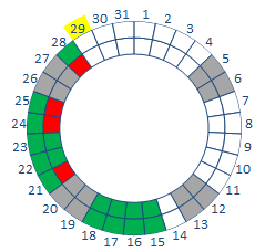
上图是该的圆环的示意图,手动制作圆环并不复杂,关键是如何利用VBA程序自动控制圆环。这里面有3点很重要:一是系统如何找到这个圆环图;二是系统如何识别内圆环还是外圆环;三是系统如何定位该月的具体哪一天。
下面将就如何消除颜色来讲解:
Sub ColorRemoval() ‘清除所有圆环的颜色
‘ActiveSheet.ChartObjects("Graphique " & i).Activate ‘系统找到该excel里面的第i个圆环图表,手动点击图表(在单元格属性里可以找到其图表名称)
’ActiveChart.FullSeriesCollection(k).Select ‘系统找到第i个圆环图表里面的第k个环图
’ActiveChart.FullSeriesCollection(k).Points(j).Select ‘系统找到第i个圆环图表里的第k个环图里的第j天
    ActiveSheet.ChartObjects("Graphique 1").Activate ‘系统找到圆环图Graphique1的图表
    ActiveChart.FullSeriesCollection(1).Select ‘系统找到内圆环
    With Selection.Format.Fill
        .Visible = msoTrue
        .ForeColor.ObjectThemeColor = msoThemeColorBackground1
        .ForeColor.TintAndShade = 0
        .ForeColor.Brightness = 0
        .Transparency = 0
        .Solid
    End With
    ActiveChart.FullSeriesCollection(2).Select ‘系统找到外圆环
    With Selection.Format.Fill
        .Visible = msoTrue
        .ForeColor.ObjectThemeColor = msoThemeColorBackground1
        .ForeColor.TintAndShade = 0
        .ForeColor.Brightness = 0
        .Transparency = 0
        .SolidEnd With
end sub
当原始数据发生变化,需要更新图表里的数据,比如当W23有数据,需要出现W23的数据。
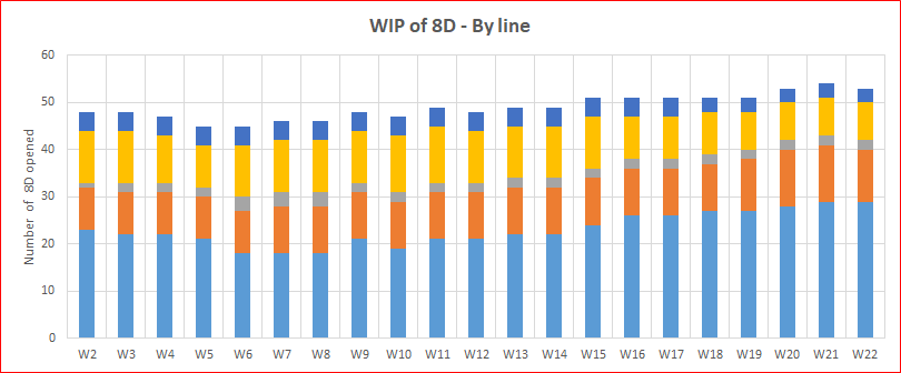
图中5种颜色分别代表不同的产品。显然,为了让数据自动刷新到新的一周,我们需要每次更新图表的数据源,否则横坐标轴无法新扩展。代码如下:
Sub refersh()

Dim col As Integer ‘value of the column
Dim Last_col As Integer ‘value of the last column
Dim nb_ligne As Integer ‘variable of the number of line of characteristics from 1 to 3
Dim the_graph As ChartObject ‘declaration of each graphic as an object in the worksheet
Dim myrange As Range
Dim WIPrange1, WIPrange2, WIPrang3, WIPrang4, WIPrang5 As Range ‘定义5种产品的
Dim i As Byte

Call DataRefresh “刷新表格的数据

i = Sheets("2018_Data_WIP").Cells(4, Columns.Count).End(xlToLeft).Column

    Do While Sheets("2018_Data_WIP").Cells(4, i) = ""
    i = i - 1
Loop

col = i - 20

Sheets("2018_Data_WIP").Activate
With Sheets("2018_Data_WIP")
    Set myrange = .Range(Cells(2, col), Cells(2, i)) ‘定义横坐标值
    WIPrange1 = .Range(Cells(4, col), Cells(4, i)) ‘对各产品,分别定义纵坐标值
    WIPrange2 = .Range(Cells(5, col), Cells(5, i))
    WIPrange3 = .Range(Cells(6, col), Cells(6, i))
    WIPrange4 = .Range(Cells(7, col), Cells(7, i))
    WIPrange5 = .Range(Cells(8, col), Cells(8, i))End With

Sheets("2018_Charts").ChartObjects.Item("chart 1").Activate ”找到图表,并且赋值
With ActiveChart
    .SeriesCollection(1).XValues = myrange
    .SeriesCollection(1).Values = WIPrange1
    .SeriesCollection(2).Values = WIPrange2
    .SeriesCollection(3).Values = WIPrange3
    .SeriesCollection(4).Values = WIPrange4
    .SeriesCollection(5).Values = WIPrange5
End With
End Sub
从上面2个例子我们可以看到如何用VBA控制图表,关键是让系统找到对应的图和点。
原文:https://www.cnblogs.com/Non-IT-developer/p/14950356.html