we can use linear model (classification)
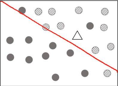
The right classification is
| striped circle | triangle |
|---|---|
| 10 | 1 |
| black circle | triangle |
|---|---|
| 11 | 1 |
but we get
| striped circle | triangle |
|---|---|
| 11 | 1 |
| black circle | triangle |
|---|---|
| 10 | 1 |
Because linear model (classification) cannot precisely classify the training set.
1.Disprove of commutative properties of matrix
Reference: https://proofwiki.org/wiki/Matrix_Multiplication_is_not_Commutative
For an order n square matrix D, let D′ be the square matrix of order n+1 defined as:
\(d_{ij}‘ =
\begin{cases}
d_{ij}: & i<n+1 \land j<n+1 \0: & i=n+1 \lor j=n+1
\end{cases}\)
Thus D′ is just D with a zero row and zero column added at the ends.
We have that D is a submatrix of D′.
Now:
\((a‘b‘)_{ij} =
\begin{cases}
\sum_{r=1}^{n+1} a‘_{ir}b‘_{rj}, & i<n+1 \land j<n+1 \0, & i=n+1 \lor j=n+1
\end{cases}\)
But:
\(\sum_{r=1}^{n+1} a‘_{ir}b‘_{rj}=a‘_{i(n+1)}b‘_{(n+1)i}+\sum_{r=1}^n a‘_{ir}b‘_{rj} \\
\qquad\qquad\quad=\sum_{r=1}^n a_{ir}b_{rj}\)
and so:
\(\mathbf{A‘B‘}(n+1,n+1)=(\mathbf{AB})‘(n+1,n+1) \\qquad\qquad\qquad\qquad=\mathbf{AB} \\qquad\qquad\qquad\qquad\neq \mathbf{BA} \\qquad\qquad\qquad\qquad= (\mathbf{BA})‘(n+1,n+1) \\qquad\qquad\qquad\qquad= \mathbf{B‘A‘}(n+1,n+1)
\)
Thus it is seen that:
\(\exists \mathbf{A‘},\mathbf{B‘}\in \mathcal{M_{n+1\times n+1}}:\mathbf{A‘B‘}\neq\mathbf{B‘A‘}\)
So \(P(k)\Rightarrow P(k+1)\) and the result follows by the Principle of Mathematical Induction
Therefore:
\(\exists \mathbf{A},\mathbf{B}\in\mathcal{M_R(n)}:\mathbf{AB}\neq\mathbf{BA}\)
2.Prove of distributive properties of matrix
Reference:https://proofwiki.org/wiki/Matrix_Multiplication_Distributes_over_Matrix_Addition
Let \(\mathbf{A}=[a]_{nn},\mathbf{B}=[b]_{nn},\mathbf{C}=[c]_{nn}\) be matrices over a ring \((\mathit{R},+,\circ)\)
Consider \(\mathbf{A}(\mathbf{B}+\mathbf{Cd})\)
Let \(\mathbf{R}=[r]_{nn}=\mathbf{B}+\mathbf{C},\mathbf{S}=[r]_{nn}=\mathbf{A}(\mathbf{B}+\mathbf{C})\)
Let \(\mathbf{G}=[g]_{nn}=\mathbf{A}\mathbf{B},\mathbf{H}=[h]_{nn}=\mathbf{A}\mathbf{C}\)
Then:
\(s_{ij}=\sum_{k=1}^n a_{ik}\circ r_{kj} \r_{kj}=b_{kj}+c_{kj} \\Rightarrow s_{ij}=\sum_{k=1}^n a_{ik}\circ(b_{kj}+c_{kj}) \\qquad =\sum_{k=1}^n a_{ik}b_{kj}+\sum_{k=1}^n a_{ik}c_{kj} \\qquad =g_{ij}+h_{ij}\)
Thus:
\(\mathbf{A}(\mathbf{B}+\mathbf{C})=(\mathbf{A}\mathbf{B})+(\mathbf{A}\mathbf{C})\)
A similar construction shows that:
\((\mathbf{B}+\mathbf{C})\mathbf{A}=(\mathbf{B}\mathbf{A})+(\mathbf{C}\mathbf{A})\)
3.Prove of associative properties of matrix
Reference:https://proofwiki.org/wiki/Matrix_Multiplication_is_Associative
Let \(\mathbf{A}=[a]_{nn},\mathbf{B}=[b]_{nn},\mathbf{C}=[c]_{nn}\) be matrices
From inspection of the subscripts, we can see that both \((\mathbf{A}\mathbf{B})\mathbf{C}\) and \(\mathbf{A}(\mathbf{B}\mathbf{C})\) are defined
Consider\((\mathbf{A}\mathbf{B})\mathbf{C}\)
Let \(\mathbf{R}=[r]_{nn}=\mathbf{A}\mathbf{B},\mathbf{S}=[s]_{nn}=\mathbf{A}(\mathbf{B}\mathbf{C})\)
Then:
\(s_{ij}=\sum_{k=1}^n r_{ik}\circ c_{kj} \r_{ik}=\sum_{l=1}^n a_{il}\circ b_{lk} \\Rightarrow s_{ij}=\sum_{k=1}^n (\sum_{l=1}^n a_{il}\circ b_{lk})\circ c_{kj} \\qquad=\sum_{k=1}^n\sum_{l=1}^n (a_{il}\circ b_{lk})\circ c_{kj}\)
Now consider \(\mathbf{A}(\mathbf{B}\mathbf{C})\)
Let \(\mathbf{R} = [r]_{nn} = \mathbf{B}\mathbf{C},\mathbf{S}=[s]_{nn}=\mathbf{A}(\mathbf{B}\mathbf{C})\)
Then:
\(s_{ij}=\sum_{l=1}^n a_{il}\circ r_{lj} \r_{lj}=\sum_{k=1}^n b_{lk}\circ c_{kj} \\Rightarrow s_{ij}=\sum_{l=1}^n a_{il}(\sum_{k=1}^n \circ b_{lk})\circ c_{kj} \\qquad=\sum_{l=1}^n\sum_{k=1}^n a_{il}\circ(b_{lk}\circ c_{kj})\)
Using Ring Axiom M1: Associativity of Product:
\(s_{ij} = \sum_{k=1}^n\sum_{l=1}^n (a_{il}\circ b_{lk})\circ c_{kj} = \sum_{l=1}^n\sum_{k=1}^n a_{il}\circ(b_{lk}\circ c_{kj})=s‘_{ij}\)
It is concluded that:
\((\mathbf{A}\mathbf{B})\mathbf{C}=\mathbf{A}(\mathbf{B}\mathbf{C})\)
\(A^{-1}=\frac{1}{|A|}A^* \A^*=\begin{bmatrix}
A_{11} & A_{21} & A_{31} \A_{12} & A_{22} & A_{32} \A_{13} & A_{23} & A_{33}
\end{bmatrix}\)
\(A_{xx}\) is algebraic complement. After calculating:
\(A^*=\begin{bmatrix}
c & -a & ad-bc \-1 & 1 & b-d \0 & 0 & c-a
\end{bmatrix}\)
\(|A|=c+0+0-(0+0+a)=c-a\)
only when \(c-a\neq 0\), A is invertible, b can be any value.
so
\(A^{-1}=\frac{1}{c-a}\begin{bmatrix}
c & -a & ad-bc \-1 & 1 & b-d \0 & 0 & c-a
\end{bmatrix}\)
If we change the matrix to
\(A = \begin{bmatrix}
2 & 2 & 3 \0 & 1 & 0 \8 & 3 & 12
\end{bmatrix}\)
\(|A|=2\times1\times2+0+0-3\times1\times8-0-0 = 0\)
When \(|A|=0\), it is not invertible.
Left-Pseudo Inverse:
\(\color{red}{\mathbf{J‘}}\mathbf{J}=\color{red}{\mathbf{(J^T J)^{-1}J^T}}\mathbf{J}=\mathbf{I_m}\)
Works if J has full column rank
Right-Pseudo Inverse:
\(\mathbf{J}\color{red}{\mathbf{J‘}}=\mathbf{J}\color{red}{\mathbf{J^T(J J^T )^{-1}}}=\mathbf{I_n}\)
Works if J has full row rank
Given \(A \in \mathbb{R}^{2\times3}\)
First calculate dimensionality of left-pseudo
\(\color{red}{\mathbf{(J^T J)^{-1}J^T}}=(\mathbb{R}^{3\times2}\mathbb{R}^{2\times3})^{-1}\mathbb{R}^{3\times2} \\qquad\qquad\quad=\mathbb{R}^{3\times2}\)
Second calculate dimensionality of right-pseudo
\(\color{red}{\mathbf{J^T(J J^T )^{-1}}} = \mathbb{R}^{3\times2}(\mathbb{R}^{2\times3}\mathbb{R}^{3\times2})^{-1} \\qquad\qquad\quad=\mathbb{R}^{3\times2}\)
So left and right pseudo invert exist
(1) \(T = wv^{-1}\\quad=\begin{bmatrix}
2 & 3 \3 & 4
\end{bmatrix}
\begin{bmatrix}
1 & 0 \0 & 1
\end{bmatrix}^{-1} \\quad=\begin{bmatrix}
2 & 3 \3 & 4
\end{bmatrix}\)
(2) \(v = Yw \Y = \begin{bmatrix}
2 & 3 \3 & 4
\end{bmatrix} \w = Y^{-1}v \=\begin{bmatrix}
2 & 3 \3 & 4
\end{bmatrix}^{-1}
\begin{bmatrix}
2 \5
\end{bmatrix}
=\begin{bmatrix}
-4 & 3 \3 & -2
\end{bmatrix}
\begin{bmatrix}
2 \5
\end{bmatrix}
=\begin{bmatrix}
7 \-4
\end{bmatrix}\)
(1)
Expectation:
\(\mathbb{E}_{x\sim p(x)} = \mathbb{E}_{x}[f] = \mathbb{E}[f] =
\begin{cases}
\sum_{x} p(x)f(x), & \text{discrete case} \\int p(x)f(x)\,{\rm d}x & \text{continuous case}
\end{cases}
\)
Variance:
\(var[x] = \mathbb{E}[(x - \mathbb{E}[x])^2] = \mathbb{E}[x^2] - \mathbb{E}[x]^2\)
Expectation is not a linear operator. However variance is a linear operator.
(2)
Estimate the expectation:
\(E(A) = 1\times1+5\times2+6\times3+3\times4+2\times5+1\times6 = 57 \E(B) = 6\times1+1\times2+1\times3+4\times4+1\times5+5\times6 = 62 \E(C) = 3\times1+2\times2+3\times3+3\times4+4\times5+3\times6 = 66\)
Estimate the variance:
\(\mu = 3\), so
\(var(A) = \frac{[(1-3)^2+(5-3)^2+(6-3)^2+(3-3)^2+(2-3)^2+(1-3)^2]}{5} = 4.4 \var(B) = \frac{[(6-3)^2+(1-3)^2+(1-3)^2+(4-3)^2+(1-3)^2+(5-3)^2]}{5} = 5.2 \var(C) = \frac{[(3-3)^2+(2-3)^2+(3-3)^2+(3-3)^2+(4-3)^2+(3-3)^2]}{5} = 0.4\).
(3) don‘t know
To do
(1)
p(back): Probability that a person has back pain
p(cold): Probability that a person has a cold
p(ncold): Probability that a person doesn‘t have a cold
(2) \(x\in N\)
(3)
\(p(cold) = 4\% \p(back|cold) = 25\% \p(back|ncold) = 10\%\)
(4)
\(p(cold|back) = \frac{p(cold,back)}{p(back)} \\qquad\qquad=\frac{p(back|cold)p(cold)}{p(back|cold)+p(back|ncold)} \\qquad\qquad=\frac{25\%\times4\%}{25\%+10\%} \\qquad\qquad=2.86\%\)
(1)
\(mutated = 42\%+2.6\% = 44.6\% \unmutated = 58\%-2.6\% = 55.4\%\)
\(\begin{array}{c|ccc}
State & \text{m} & \tilde{m}\\hline
\tilde{m} & 44.6\% & 55.4\% \\end{array}\)
(2)
import numpy as np
import matplotlib.pyplot as plt
# State space
states = ["Mutated","Unmutated"]
# Possible events
transitionName = [["UM","UU"],["MU","MM"]]
# Probilistic matrix
transitionMatrix = [0.446,0.554]
def activity_forecast(days):
# Choose initial state
activityToday = "Unmutated"
print("Start state: " + activityToday)
# Initial state list
activityList = [activityToday]
prob_list = []
i = 0
# Calculate the probability of activityList
prob = 1
while i != days:
if activityToday == "Unmutated":
change = np.random.choice(transitionName[0],replace=True,p=transitionMatrix)
if change == "UM":
prob = prob * 0.446
activityToday = "Mutated"
activityList.append("Mutated")
prob_list.append(prob)
pass
elif change == "UU":
prob = prob * 0.554
activityList.append("Unmutated")
prob_list.append(prob)
elif activityToday == "Mutated":
change = np.random.choice(transitionName[1], replace=True, p=transitionMatrix)
if change == "MU":
prob = prob * 0.446
activityToday = "Unmutated"
activityList.append("Unmutated")
prob_list.append(prob)
pass
elif change == "MM":
prob = prob * 0.554
activityList.append("Mutated")
prob_list.append(prob)
i += 1
print("Possible states: " + str(activityList))
print("End state after "+ str(days) + " days: " + activityToday)
print("Probability of the possible sequence of states: " + str(prob))
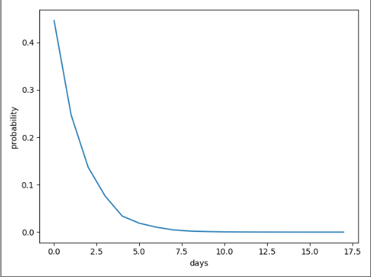
x = np.arange(0, 18, 1)
prob_list = np.array(prob_list)
plt.plot(x,prob_list)
plt.show()
# predict states after 18 days
activity_forecast(18)
The result is
Start state: Unmutated
Possible states: [‘Unmutated‘, ‘Unmutated‘, ‘Mutated‘, ‘Unmutated‘, ‘Unmutated‘, ‘Mutated‘, ‘Mutated‘, ‘Unmutated‘, ‘Unmutated‘, ‘Unmutated‘, ‘Unmutated‘, ‘Mutated‘, ‘Unmutated‘, ‘Mutated‘, ‘Mutated‘, ‘Mutated‘, ‘Mutated‘, ‘Unmutated‘, ‘Mutated‘]
End state after 18 days: Mutated
Probability of the possible sequence of states: 3.432429382297346e-06
Plot:
(3) don‘t know
To do
(1)
Measure the information in single:
\(h(p_i) = -\log_{2} p_i\)
So
\(h(S_1) = -\log_{2} 0.04 = 4.64 \h(S_2) = -\log_{2} 0.22 = 2.18 \h(S_3) = -\log_{2} 0.67 = 0.58 \h(S_4) = -\log_{2} 0.07 = 3.83 \\\)
(2)
Measure average information:
\(H(p) = \mathbb{E}[h(.)] = \sum_{i} p_i h(p_i) = -\sum_{i} p_i \log_{2} p_i\)
So the entropy is
\(0.04\times4.64 + 0.22\times2.18 + 0.67\times0.58 + 0.07\times3.83 \=1.3219\)
Bayes Decision Theory describes the probability of an event, based on prior knowledge of conditions that might be related to the event.
Its Goal is to minimize the misclassification rate.
Bayes optimal classification based on probability distributions \(p(x|C_k)p(C_k)\)
We compare the result among the magnitude of \(p(x|C_1)\) and \(p(x|C_2)\)
Who is bigger, then we choose it. For example, when \(p(x|C_1)\) is bigger, then we choose \(C_1\)
\(p(x|C_1) = \frac{p(xC_1)}{p(C_1)} = \frac{p(C_1|x)p(x)}{p(C_1)}\p(x|C_2) = \frac{p(xC_2)}{p(C_2)} = \frac{p(C_2|x)p(x)}{p(C_2)}\)
Because \(p(C_1) = p(C_2)\) and \(\sigma_1 = \sigma_2\)
According to Gaussian Distribution so \(\mu_1 = \mu_2\)
So \(p(x|a) = p(x|b)\)
Then \(p(xa) = p(xb)\)
So \(x^* = \mu_1 \quad \text{or} \quad \mu_2\)
lecture_04_bayesian_decision_theory page 17
原文:https://www.cnblogs.com/Java-Starter/p/14775184.html