1-手动线性回归

import torch
from matplotlib import pyplot as plt
import random
import traceback

# create data
def create_data(W, b, num):
    X = torch.normal(mean=0, std=1, size =(num, len(W)))
    y = X.matmul(W) + b
    # 加点噪声
    y += torch.normal(mean=0, std=0.1, size=(num,))
    return X, y 

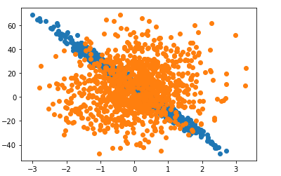
def plot_scatt(x, y):
    plt.scatter(x, y)
                      
W_true = torch.tensor([3, -20.5])
b_true = 8
data_num = 1000
features, labels = create_data(W_true, b_true, data_num)
plot_scatt(features[:, 1], labels)
plot_scatt(features[:, 0], labels)

def get_batch(X, y, batch_size):
    input_size = len(X) 
    index = list(range(input_size))
    random.shuffle(index)
    for i in range(0, input_size, batch_size):
        batch_indices = torch.tensor(index[i: min(batch_size+i, input_size)])
        yield X[batch_indices], y[batch_indices]

import math

W = torch.normal(mean=0, std=0.01, size=(2,1), requires_grad=True)
b = torch.zeros(1, requires_grad=True)

# model
def target_func(X, W, b):
    return X.matmul(W) + b

# loss
def cal_loss(y, y_, batch_size):
#     print(y, y_, batch_size)
    return ((y - y_.reshape(y.shape)) ** 2 /2).sum()/batch_size

# sgd
def sgd(params, lr):
    with torch.no_grad():
        for param in params:
            param -= lr * param.grad
            param.grad.zero_()
    

# 训练过程
epochs = 30
batch_size = 10
lr = 0.003
for i in range(epochs):
    for X, y in get_batch(features, labels, batch_size):
        loss = cal_loss(y, target_func(X, W, b), batch_size)
        loss.backward()
        sgd([W, b], lr)
    with torch.no_grad():
        loss = cal_loss(labels, target_func(features, W, b), len(labels))
        print("loss", loss)
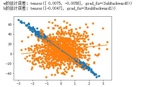
print(f‘w的估计误差: {W_true - W.reshape(W_true.shape)}‘)
print(f‘b的估计误差: {b_true - b}‘)

def plot_linear(x, y, w, b):
    plt.scatter(x, y)
    yy_list = []
    for xx in x:
        yy_list.append(w * xx.item() +b.item())
#     print(yy_list)
    plt.plot(x, yy_list)
    
# print(W[1].item())
plot_linear(features[:, 1], labels, W[1].item(), b)
plot_linear(features[:, 0], labels, W[0].item(), b)