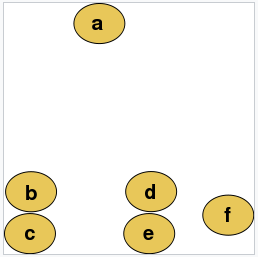
层次聚类的策略一般分为两类
Agglomerative: This is "bottom-up" approach: each observation starts in its own cluster, and pairs of clusters are merged as one moves up the hierarchy.
这是一种“自底向上”的方法:每个观测值都是单独的一个簇,并且当一个簇向上移动时,成对的簇被合并为一个簇。
Divisive: This is a "top-down" approach: all observations start in one cluster, and splits are performed recursively as one moves down the hierarchy.
这是一种“自顶向下”的方法:所有的观测都从一个簇开始,当一个观察向下移动时,递归地执行分裂为多个簇。
The standard algorithm for hierarchical agglomerative clustering (HAC) has a time complexity of \(O(n^3)\) and requires \(O(n^2)\) memory, which makes it too slow for even medium data sets.
标准的层次聚类算法(自底向上)需要\(O(n^3)\)的时间,\(O(n^2)\)的空间。
For text or other non-numeric data, metrics such as the Hamming distance or Levenshtein distance are often used.
对于文本或其他非数字数据,通常使用诸如Hamming距离或Levenshtein距离之类的度量。
链接标准用于确定两个观测集合之间的距离计算。
The linkage criterion determines the distance between sets of observations as a function of the pairwise distances between observations.
常见的链接标准有:
| Names | Formula |
|---|---|
| Maximum or complete-linkage clustering | \(max(d(a,b):a \in A, b\in B)\) |
| Minimum or single-linkage clustering | \(min(d(a,b):a \in A, b\in B)\) |
| Unweighted average linkage clustering (or UPGMA) | \(\frac{1}{\|A\|\cdot \|B\|}\sum_{a\in A}\sum_{b\in B}d(a,b)\) |
| Names | Formula |
|---|---|
| 完全(最远)链接聚合聚类 | \(max(d(a,b):a \in A, b\in B)\) |
| 单连接(最近)聚合聚类 | \(min(d(a,b):a \in A, b\in B)\) |
| 平均聚合聚类 | \(\frac{1}{\|A\|\cdot \|B\|}\sum_{a\in A}\sum_{b\in B}d(a,b)\) |
Example
Agglomerative clustering example
For example, suppose this data is to be clustered, and the Euclidean distance is the distance metric.
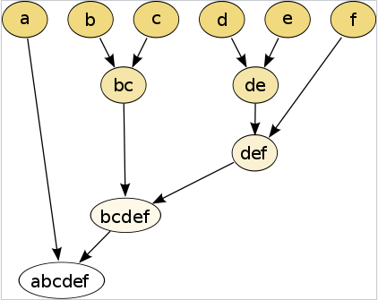
UPGMA (unweighted pair group method with arithmetic mean) is a simple agglomerative (bottom-up) hierarchical clustering method.
UPGMA是一种简单的聚合型(自底向上)层次聚类方法。
第一步:
我们假设我们有5个元素,和他们两两之间距离矩阵。
| a | b | c | d | e | |
|---|---|---|---|---|---|
| a | 0 | 17 | 21 | 31 | 23 |
| b | 17 | 0 | 30 | 34 | 21 |
| c | 21 | 30 | 0 | 28 | 39 |
| d | 31 | 34 | 28 | 0 | 43 |
| e | 23 | 21 | 39 | 43 | 0 |
在这个例子中,\(D_1 (a,b) = 17\)是最小的值,所以我们首先合并元素a和b。
First branch length estimation
第一次分支长度估算
假设 \(u\) 当做连接a和b的节点,有\(\delta(a,u)=\delta(b,u)=D_1(a,b)/2=8.5\).
因此连接a,b与 \(u\) 的分支长度为8.5
First distance matrix update
第一次距离矩阵更新
第二步:
更新之后的距离矩阵
| (a,b) | c | d | e | |
|---|---|---|---|---|
| (a,b) | 0 | 25.5 | 32.5 | 22 |
| c | 25.5 | 0 | 28 | 39 |
| d | 32.5 | 28 | 0 | 43 |
| e | 22 | 39 | 43 | 0 |
(a,b) 与 e 的距离最小,所以合并这两个元素
Second branch length estimation
第二次分支长度估算
假设 \(v\) 当做连接(a,b)和e的节点,有
\(\delta(a,v)=\delta(b,v)=\delta(e,v)=D_2((a,b),e)/2=11\)
\(\delta(u,v)=\delta(e,v)-\delta(a,u) = 11-8.5 = 2.5\)
因此连接a,b与 \(u\) 的分支长度为8.5
Second distance matrix update
第二次距离矩阵更新
第三步:
| ((a,b),e) | c | d | |
|---|---|---|---|
| ((a,b),e) | 0 | 30 | 36 |
| c | 30 | 0 | 28 |
| d | 36 | 28 | 0 |
c和d的距离最小,合并cd
Third branch length estimation
第三次分支长度估算
\(\delta(c,w)=\delta(d,w)=D_1(c,d)/2=14\)
Third distance matrix update
第三次距离矩阵更新
第四步
| ((a,b),e) | (c,d) | |
|---|---|---|
| ((a,b),e) | 0 | 33 |
| (c,d) | 33 | 0 |
直接合并两个节点
最终生成的树
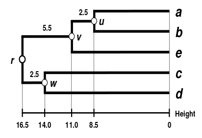
其中每个节点到根节点的距离是一样的。
原文:https://www.cnblogs.com/XiiX/p/14642632.html