该比赛将使用具有挑战性的时间序列数据集,由俄罗斯最大的软件公司之一 1C公司提供。数据中包括商店,商品,价格,日销量等连续34个月的数据,要求预测第35个月产品和商店的销量。评价指标为RMSE,Baseline是1.1677。
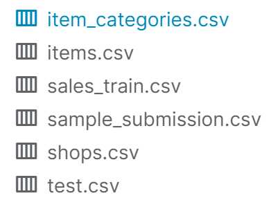
数据集共6张表。其中sales_train是主表。item_categories, items, shops为补充表。test为提交用的表,sample_submission表顾名思义。
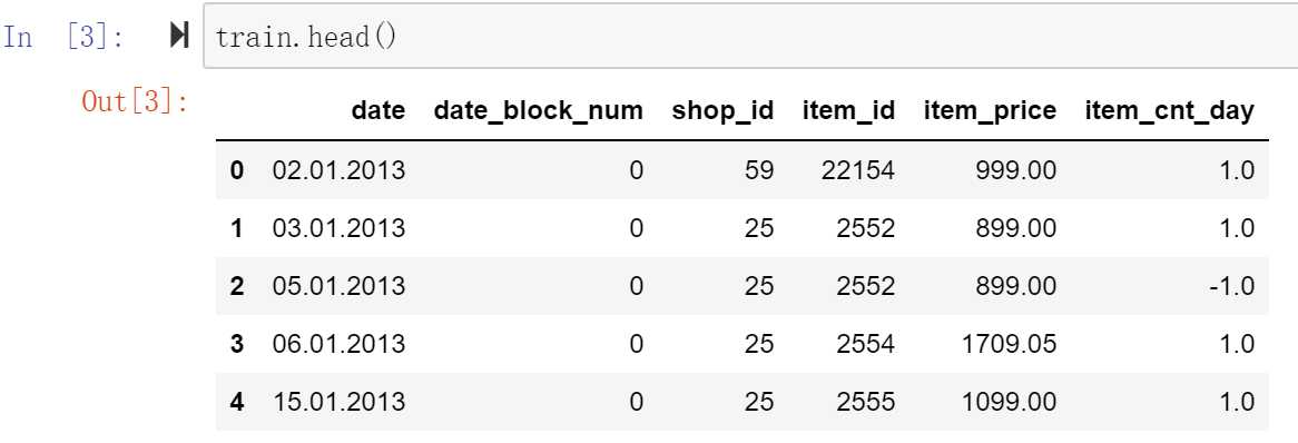
拿到数据后,先看一下数据。csv数据直接用pd.read_csv来阅读,pd.head()可看到该pd的前5行数据,pd.info()可统计该pd属性type、count等信息,df.describe()可统计pd中每个属性mean、std等信息。

train = pd.read_csv("../DATA/SALES/sales_train.csv")
cats = pd.read_csv("../DATA/SALES/item_categories.csv")
items = pd.read_csv("../DATA/SALES/items.csv")
shops=pd.read_csv("../DATA/SALES/shops.csv")
test = pd.read_csv("../DATA/SALES/test.csv")
大概探索一下这些表,可知:
共2935849行数据,有date,date_block_num(月份count),shop_id, item_id, item_price, item_cnt_day(每天销量,转成每月后就是 target_y)。
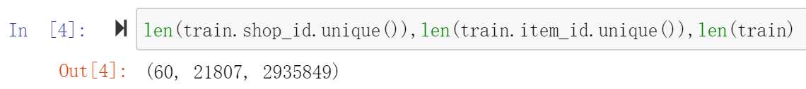
其中shop_id共有60个不重复的值,item_id有21807个不重复的值。如果所有shop_id和item_id进行组合的话,会有 60 * 21807 * 33(月份)= 43177860。远大于sales_train表中的数字。说明sales_train中的表是不全的。可能是1)商店确实没有卖这个商品;2)有这个商品但是卖出是0,就没有记录。
用代码验证后发现,item_cnt_day确实没有等于0的数据。说明第二种情况肯定是存在的。因为一个商店卖的商品,不可能所有商品每天一定都会有卖出。
仔细再想一下第一种情况,商店没有卖这个商品,那么卖出肯定也是0,和第二种情况也不冲突。所以即使商店没有卖这种商品,也可以把它补全成卖出数量为0。同时可以再给数据增加一个特征,表明该商店有卖出过商品,还是从未卖过该商品。
所以我们需要自己补全train表中所有shop_id和item_id的组合,没有卖出也是一个重要信息,千万不能忽视了。
其中,
item_price和item_cnt_day是和 target_y 比较直接相关的两个连续特征,用sns画一下joinplot看一下:
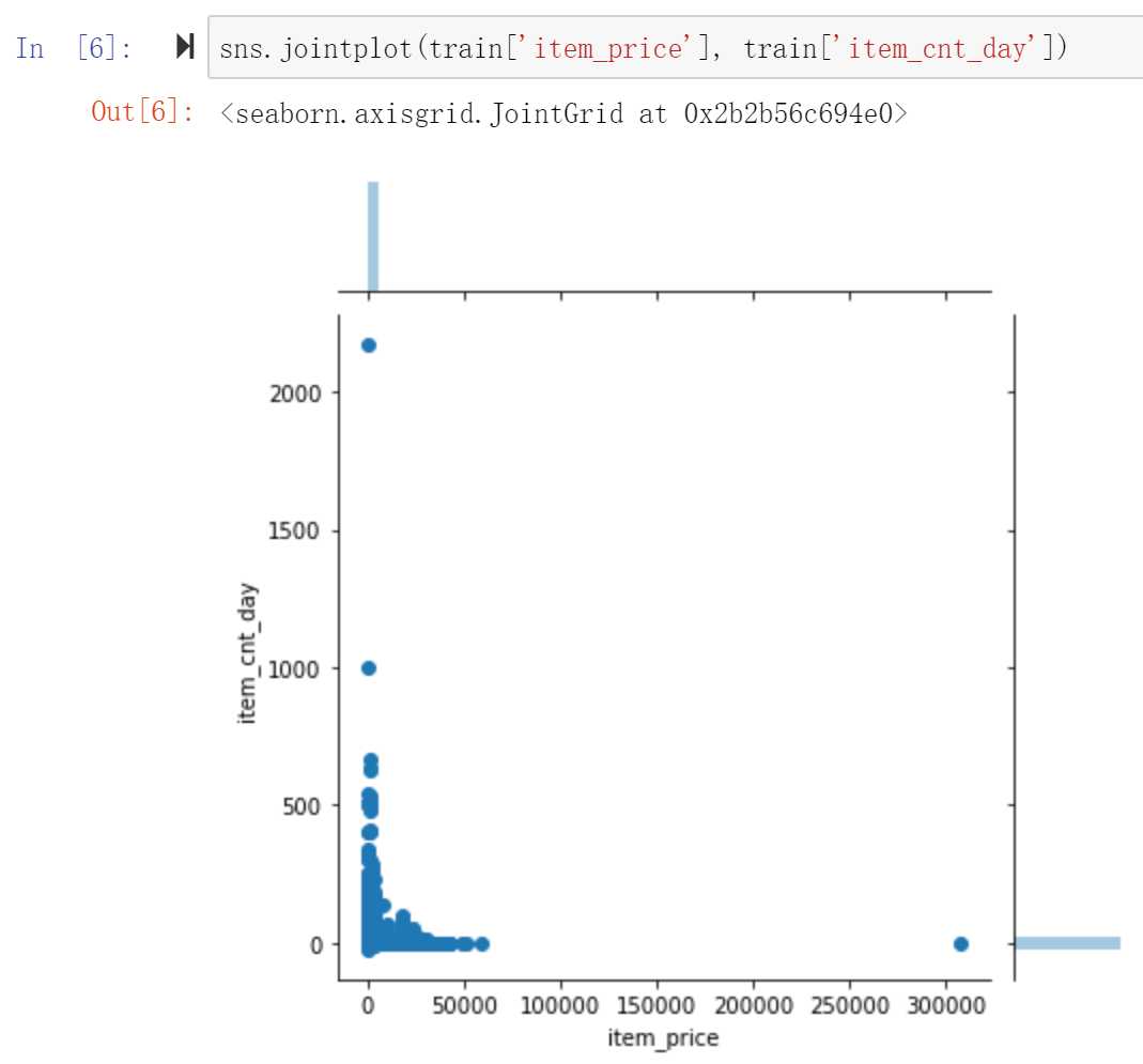
可以看到item_cnt_day和item_price都存在一些离群点,如果直接放到模型中训练,可能会造成训练数据的偏差。所以要把离群点去掉。
train = train[train.item_cnt_day<=1000]
train = train[(train.item_price<100000) & (train.item_price>0)]
共2w余行数据,有item_name, item_id, item_category_id
item的类别特征通过item_categories表已经可以得到了。item_name没有看出什么特别用处,所以先去掉。
items.drop([‘item_name‘],axis=1,inplace=True)
共84行,有item_category_name(包含商品大类别,小类别,可拆分后通过item_id补充到sales_train中),item_category_id
item_category_name中有一些名字有双引号,把双引号先去掉,规范命名。
cats[‘item_category_name‘] = cats[‘item_category_name‘].str.replace(‘"‘,‘‘)
仔细观察item_category_name的命名规则,可以发现它的命名里面是包含了商品大类别和小类别,用“-”来分隔的。
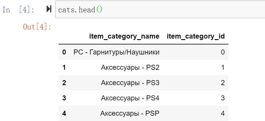
所以我们可以把它们拆分出来作为补充特征,拉近某些商品之间的关联,比如在同一个大类别下面肯定更近一些。
cats[‘split_name‘] = cats[‘item_category_name‘].str.split(‘-‘)
cats[‘item_type‘] = cats[‘split_name‘].map(lambda x:x[0].strip())

cats[‘item_subtype‘] = cats[‘split_name‘].map(lambda x:x[1].strip() if len(x)>1 else x[0].strip())

# label encoder
cats[‘item_type‘] = LabelEncoder().fit_transform(cats[‘item_type‘])
cats[‘item_subtype‘] = LabelEncoder().fit_transform(cats[‘item_subtype‘])
cats = cats[[‘item_category_id‘,‘item_type‘,‘item_subtype‘]]
共60行,有shop_name(包含地区信息,商店类别信息可拆解后通过shop_id补充到sales_train中), shop_id
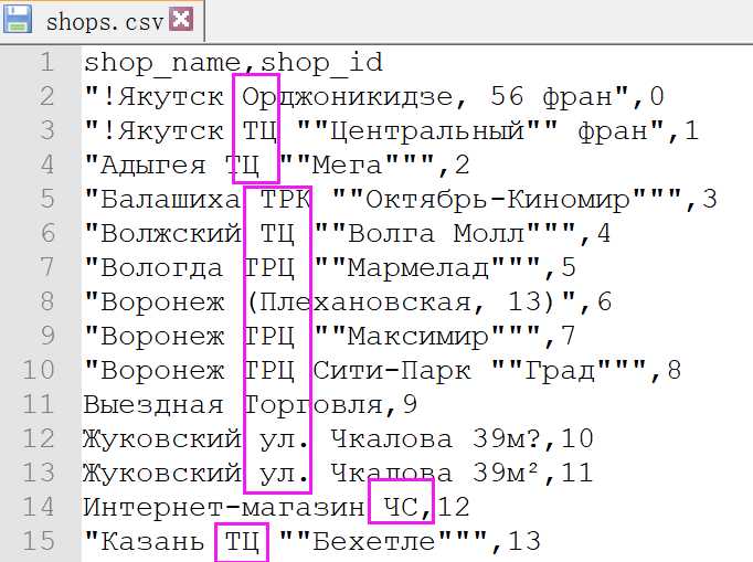
观察(其实是谷歌翻译后)可发现,shop_name中的命名规律是第一个单词城市名,第二个单词很多商店是重复的,应该就是商店的类型,后面跟的应该就是商店的地址。所以可提取商店的城市和类型出来,使不同商店有一些的相关性。
1 shops[‘city‘] = shops[‘shop_name‘].str.split(‘ ‘).map(lambda x: x[0])
2 shops[‘shop_city‘] =  LabelEncoder().fit_transform(shops[‘city‘])
3
4 shops[‘shop_type‘] = shops[‘shop_name‘].str.split(‘ ‘).map(lambda x: x[1] if len(x)>2 else ‘None‘)
5 shops[‘shop_type‘] =  LabelEncoder().fit_transform(shops[‘shop_type‘])
6
7 shops = shops[[‘shop_id‘,‘shop_city‘,‘shop_type‘]]
共20w行,有shop_id, item_id。只有这两个属性肯定是不能很好的预测的,所以要对test先进行补充。即根据其他表数据里对应的shop_id, item_id去补充test数据。
探索一下test表可发现:
test表中共5100个item_id,42个shop_id, 其中有363个item_id从未在train set中出现过,所有shop_id都在train_set中出现过。
由上可知,sale_train.csv可以通过shop_id、item_id、item_category_id来合并items.csv、item_categories.csv和shops.csv。test.csv也可根据shop_id, item_id进行扩充。下一步就是merge tables
1. 对于train表(原sales_train表),1)补足商店没有售出商品的shop_item组合,没有售出本身也是一种数据;2)生成item_cnt_month
 1 # add item_cnt_month
 2 tmp_df = train.groupby([‘date_block_num‘,‘shop_id‘,‘item_id‘]).agg({‘item_cnt_day‘:‘sum‘, ‘item_price‘:‘mean‘})
 3 tmp_df.columns = pd.Series([‘item_cnt_month‘, ‘item_month_avg_price‘])
 4 tmp_df.reset_index(inplace=True)
 5
 6 # 用join会提示特征名一致的报错,用merge更方便一点
 7 train_df = pd.merge(train_df, tmp_df, on=[‘date_block_num‘,‘shop_id‘,‘item_id‘],
 8                    how=‘left‘)
 9
10 train_df[‘item_month_avg_price‘] = train_df[‘item_month_avg_price‘].fillna(0).astype(np.float32)
11 train_df[‘item_cnt_month‘] = train_df[‘item_cnt_month‘].fillna(0).astype(np.float16)
注:把item_cnt_month剪裁到20内。这个是题目里给出的条件,很重要!

我就是一开始没注意这个,后来加上这个crop后,loss马上就从1.多掉到0.9多了 :P
##### 剪到20里面,这个很重要
train_df[‘item_cnt_month‘] = train_df[‘item_cnt_month‘].clip(0,20)
2. 把test表接到train后面,这样可以一起和其他表merge,补其他特征。test表的date_block_num是34.
test[‘date_block_num‘] = 34
test[‘date_block_num‘] = test[‘date_block_num‘].astype(np.int8)
test[‘shop_id‘] = test[‘shop_id‘].astype(np.int8)
test[‘item_id‘] = test[‘item_id‘].astype(np.int16)

df = pd.concat([train_df, test], ignore_index=True, sort=False,
                keys=[‘date_block_num‘,‘shop_id‘,‘item_id‘])

df.fillna(0, inplace=True)
3. merge其他表,补齐相关特征。我一开始用的join,会报两个表中有column name相同的报错。所以还是用merge会方便一些。
# shop
df = pd.merge(df, shops, on=‘shop_id‘,how=‘left‘)
# item
df = pd.merge(df, items, on=‘item_id‘,how=‘left‘)
# item_category
df = pd.merge(df, cats, on=‘item_category_id‘,how=‘left‘)
4. 调优,下面这些是后来提交结果后结果不够好,又反过头来调优时发现的:
item_category表中,item_type有重复的,可合并:
 1 cats[‘item_category_name‘] = cats[‘item_category_name‘].str.replace(‘"‘,‘‘)
 2
 3 cats[‘split_name‘] = cats[‘item_category_name‘].str.split(‘-‘)
 4 cats[‘item_type‘] = cats[‘split_name‘].map(lambda x:x[0].strip())
 5
 6 map_dict = {
 7     ‘PC‘:‘Аксессуары‘,
 8     ‘Чистые носители (шпиль)‘:‘Чистые носители‘,
 9     ‘Чистые носители (штучные)‘: ‘Чистые носители‘
10
11 }
12 cats[‘item_type‘] = cats[‘item_type‘].apply(lambda x:map_dict[x] if x in map_dict.keys() else x)
13
14 cats[‘item_subtype‘] = cats[‘split_name‘].map(lambda x:x[1].strip() if len(x)>1 else x[0].strip())
15
16 # label encoder
17 cats[‘item_type‘] = LabelEncoder().fit_transform(cats[‘item_type‘])
18 cats[‘item_subtype‘] = LabelEncoder().fit_transform(cats[‘item_subtype‘])
19 cats = cats[[‘item_category_id‘,‘item_type‘,‘item_subtype‘]]
shop表中,有shop_name是一样的,可合并:
 1 # shops中shop_name第10、11一样,可去掉第10个shop。0和57,1和58仅后缀不一样。
 2 # 直接修改train、test中的shop_id即可,因为最终还是要join到train上
 3 train.loc[train.shop_id == 10, ‘shop_id‘] = 11
 4 test.loc[test.shop_id == 10, ‘shop_id‘] = 11
 5
 6 train.loc[train.shop_id == 0, ‘shop_id‘] = 57
 7 test.loc[test.shop_id == 0, ‘shop_id‘] = 57
 8
 9 train.loc[train.shop_id == 1, ‘shop_id‘] = 58
10 test.loc[test.shop_id == 1, ‘shop_id‘] = 58
11
12 train.loc[train.shop_id == 40, ‘shop_id‘] = 39
13 test.loc[test.shop_id == 40, ‘shop_id‘] = 39
14
15 shops.drop([0,1,10],axis=0,inplace=True)
此时,train数据包括test数据,重命名为 df 表后的情况如下:
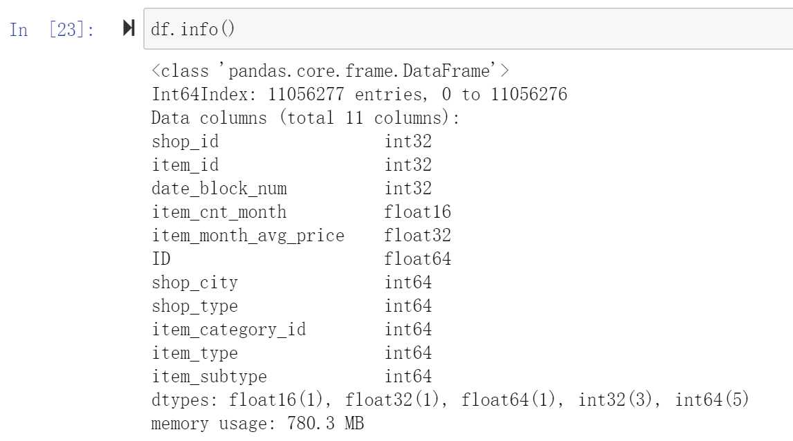
5. 调整一下数据精度,能调小的都尽量调小成int8 / int16。
不然内存可能会用爆(在后面组合特征算lag时,别问我怎么知道会爆,问就是我爆了才知道的。。不过我后来发现我内存用爆主要是因为我做lag特征时,没有去重。)
df[‘shop_id‘] = df[‘shop_id‘].astype(np.int8)
df[‘item_id‘] = df[‘item_id‘].astype(np.int16)
df[‘date_block_num‘] = df[‘date_block_num‘].astype(np.int8)
df[‘item_cnt_month‘] = df[‘item_cnt_month‘].astype(np.float16)
df[‘item_month_avg_price‘] = df[‘item_month_avg_price‘].astype(np.float32)
df[‘shop_city‘] = df[‘shop_city‘].astype(np.int8)
df[‘shop_type‘] = df[‘shop_type‘].astype(np.int8)
df[‘item_category_id‘] = df[‘item_category_id‘].astype(np.int8)
df[‘item_type‘] = df[‘item_type‘].astype(np.int8)
df[‘item_subtype‘] = df[‘item_subtype‘].astype(np.int8)
这个项目的target是一个有时间依赖的问题。当前月的销售量,可以参考之前一个月、两个月...的销售量数据。商品售价也不是一尘不变的,同样会有一些时序上的趋势特征。所以我们需要自己构造lag features。例如把一个月前的销售量作为特征加到当前这个月里。
lag function
 1 # 考虑历史数值
 2 def lag_feature(df, lag_range, shift_feature):
 3     tmp = df[[‘date_block_num‘,‘shop_id‘,‘item_id‘,shift_feature]]
 4     for lag in lag_range:
 5         #print(‘processing lag:‘,lag)
 6         #### drop duplicate很重要 ######
 7         shifted_df = tmp.copy().drop_duplicates()
 8         shifted_df.columns = [‘date_block_num‘,‘shop_id‘,‘item_id‘,shift_feature+‘_lag_‘+str(lag)]
 9         shifted_df[‘date_block_num‘] += lag
10         df = pd.merge(df, shifted_df, on=[‘date_block_num‘, ‘shop_id‘, ‘item_id‘], how=‘left‘)
11     df = df.fillna(0)
12     return df
lag features
 1 # item_cnt_month
 2 df = lag_feature(df, [1,2,3], ‘item_cnt_month‘)
 3
 4 #item_price_month
 5 tmp = df.groupby([‘date_block_num‘,‘item_id‘]).agg({‘item_cnt_month‘:‘mean‘})
 6 tmp.columns = pd.Series([‘item_avg_month‘])
 7 tmp.reset_index(inplace=True)
 8 df = pd.merge(df, tmp, how=‘left‘, on=[‘date_block_num‘,‘item_id‘])
 9
10 df = lag_feature(df, [1,2,3], ‘item_avg_month‘)
11 df.drop(‘item_avg_month‘, axis=1, inplace=True)
12
13 # shop_month
14 tmp = df.groupby([‘date_block_num‘,‘shop_id‘]).agg({‘item_cnt_month‘:‘mean‘})
15 tmp.columns = pd.Series([‘shop_cnt_month‘])
16 tmp.reset_index(inplace=True)
17 df = pd.merge(df, tmp, how=‘left‘, on=[‘date_block_num‘,‘shop_id‘])
18
19 df = lag_feature(df, [1,2,3], ‘shop_cnt_month‘)
20 df.drop(‘shop_cnt_month‘, axis=1, inplace=True)
21
22 #category_month
23 tmp = df.groupby([‘date_block_num‘,‘item_category_id‘]).agg({‘item_cnt_month‘:‘mean‘})
24 tmp.columns = pd.Series([‘category_cnt_month‘])
25 tmp.reset_index(inplace=True)
26 df = pd.merge(df, tmp, how=‘left‘, on=[‘date_block_num‘,‘item_category_id‘])
27
28 df = lag_feature(df, [1,2,3], ‘category_cnt_month‘)
29 df.drop(‘category_cnt_month‘, axis=1, inplace=True)
30
31 #big_category_month
32 tmp = df.groupby([‘date_block_num‘,‘item_type‘]).agg({‘item_cnt_month‘:‘mean‘})
33 tmp.columns = pd.Series([‘big_category_cnt_month‘])
34 tmp.reset_index(inplace=True)
35 df = pd.merge(df, tmp, how=‘left‘, on=[‘date_block_num‘,‘item_type‘])
36
37 df = lag_feature(df, [1,2,3], ‘big_category_cnt_month‘)
38 df.drop(‘big_category_cnt_month‘, axis=1, inplace=True)
39
40 #shop_city_month
41 tmp = df.groupby([‘date_block_num‘,‘shop_city‘]).agg({‘item_cnt_month‘:‘mean‘})
42 tmp.columns = pd.Series([‘shop_city_cnt_month‘])
43 tmp.reset_index(inplace=True)
44 df = pd.merge(df, tmp, how=‘left‘, on=[‘date_block_num‘,‘shop_city‘])
45
46 df = lag_feature(df, [1,2,3], ‘shop_city_cnt_month‘)
47 df.drop(‘shop_city_cnt_month‘, axis=1, inplace=True)
48
49 # shop_type_month
50 tmp = df.groupby([‘date_block_num‘,‘shop_type‘]).agg({‘item_cnt_month‘:‘mean‘})
51 tmp.columns = pd.Series([‘shop_type_cnt_month‘])
52 tmp.reset_index(inplace=True)
53 df = pd.merge(df, tmp, how=‘left‘, on=[‘date_block_num‘,‘shop_type‘])
54
55 df = lag_feature(df, [1,2,3], ‘shop_type_cnt_month‘)
56 df.drop(‘shop_type_cnt_month‘, axis=1, inplace=True)
关于lag时长的选择:
一开始我其实都是给加上了6个月的lag features,因为考虑到一个长期趋势的问题。
但是训练完,画特征重要性的图时,我发现6个月的lag特征重要性都不高。所以我后来09改成了3个月。
因为 1)6个月没啥效果;2)会损失更多数据。如果用6个月的lag feature,前0-5个月没有lag feature,会被删掉。比起3个月的lag feature就多损失了3个月的数据。
关于lag feature的调优补充:
用上面这些lag feature去训练并预测提交后,大概是0.94, 排名3338,top 40%。距离top 10%还有一定距离。所以特征还是不够好。于是又进行了下面的一些特征补充:
1)月份,天数
考虑到不同月份会有一些不同节日,对商品的售卖会有影响。比如国外12月有圣诞节,商品一般都会有一些打折,卖的也会更多。
每个月份天数不同,那么对一个月卖的商品数量也会有一些影响。比如相等条件下,28天肯定卖的比30天卖的少,这是正常的。
所以从date这个参数中提取month和days的特征。
1 # 某些月份可能会卖的更好一些,加上month特征
2 df[‘month‘] = (df[‘date_block_num‘] % 12).astype(np.int8)
3 # days
4 days = pd.Series([31,28,31,30,31,30,31,31,30,31,30,31])
5 df[‘days‘] = df[‘month‘].map(days).astype(np.int8)
2)更多的不同lag feature
1. 商品新旧程度。商品第一次进行交易的月份,反映了这个商品距离现在的新旧程度。因为test中有很多是新商品,加上这个特征后,就可以在train中得到过往的新商品的一个销售量的一些变化趋势。
 1 # 商品新旧程度
 2 first_item_block = df.groupby([‘item_id‘])[‘date_block_num‘].min().reset_index()
 3 first_item_block[‘item_first_interaction‘] = 1
 4
 5 df = pd.merge(df, first_item_block[[‘item_id‘, ‘date_block_num‘, ‘item_first_interaction‘]], on=[‘item_id‘, ‘date_block_num‘], how=‘left‘)
 6 df[‘item_first_interaction‘].fillna(0, inplace=True)
 7 df[‘item_first_interaction‘] = df[‘item_first_interaction‘].astype(‘int8‘)
 8
 9 # 1-3 months avg category sales for new items
10 item_id_target_mean = df[df[‘item_first_interaction‘] == 1].groupby([‘date_block_num‘,‘item_subtype‘, ‘shop_id‘])[‘item_cnt_month‘].mean().reset_index().rename(columns={
11     "item_cnt_month": "new_item_shop_cat_avg"}, errors="raise")
12
13 df = pd.merge(df, item_id_target_mean, on=[‘date_block_num‘,‘item_subtype‘, ‘shop_id‘], how=‘left‘)
14
15 df[‘new_item_shop_cat_avg‘] = (df[‘new_item_shop_cat_avg‘]
16                                 .fillna(0)
17                                 .astype(np.float16))
18
19 df = lag_feature(df, [1, 2, 3], ‘new_item_shop_cat_avg‘)
20 df.drop([‘new_item_shop_cat_avg‘], axis=1, inplace=True)
2. 其他shop_id, shop_city,item_category,item_id,月份的组合。和每个月的item_cnt_month的平均。
 1 # item city month
 2 tmp = df.groupby([‘date_block_num‘,‘item_id‘, ‘shop_city‘])[‘item_cnt_month‘].mean().reset_index().rename(columns={
 3     "item_cnt_month": "item_city_cnt_month"}, errors="raise")
 4
 5 df = pd.merge(df, tmp, on=[‘date_block_num‘,‘item_id‘, ‘shop_city‘], how=‘left‘)
 6
 7 df[‘item_city_cnt_month‘] = (df[‘item_city_cnt_month‘]
 8                                 .fillna(0)
 9                                 .astype(np.float16))
10
11 df = lag_feature(df, [1,2,3], ‘item_city_cnt_month‘)
12 df.drop(‘item_city_cnt_month‘, axis=1, inplace=True)
13
14 #item_shop_month
15 item_id_target_mean = df.groupby([‘date_block_num‘,‘item_id‘, ‘shop_id‘])[‘item_cnt_month‘].mean().reset_index().rename(columns={
16     "item_cnt_month": "item_shop_target_enc"}, errors="raise")
17
18 df = pd.merge(df, item_id_target_mean, on=[‘date_block_num‘,‘item_id‘, ‘shop_id‘], how=‘left‘)
19
20 df[‘item_shop_target_enc‘] = (df[‘item_shop_target_enc‘]
21                                 .fillna(0)
22                                 .astype(np.float16))
23
24 df = lag_feature(df, [1, 2, 3], ‘item_shop_target_enc‘)
25 df.drop([‘item_shop_target_enc‘], axis=1, inplace=True)
26
27 # item month
28 tmp = df.groupby([‘date_block_num‘]).agg({‘item_cnt_month‘: [‘mean‘]})
29 tmp.columns = [ ‘date_avg_item_cnt‘ ]
30 tmp.reset_index(inplace=True)
31
32 df = pd.merge(df, tmp, on=[‘date_block_num‘], how=‘left‘)
33 df[‘date_avg_item_cnt‘] = df[‘date_avg_item_cnt‘].astype(np.float16)
34 df = lag_feature(df, [1,2,3], ‘date_avg_item_cnt‘)
35 df.drop([‘date_avg_item_cnt‘], axis=1, inplace=True)
36
37 # shop_category_month
38 tmp = df.groupby([‘date_block_num‘, ‘item_category_id‘,‘shop_id‘]).agg({‘item_cnt_month‘: [‘mean‘]})
39 tmp.columns = [ ‘date_cat_shop_avg_item_cnt‘ ]
40 tmp.reset_index(inplace=True)
41
42 df = pd.merge(df, tmp, on=[‘date_block_num‘, ‘item_category_id‘,‘shop_id‘], how=‘left‘)
43 df[‘date_cat_shop_avg_item_cnt‘] = df[‘date_cat_shop_avg_item_cnt‘].astype(np.float16)
44 df = lag_feature(df, [1,2,3], ‘date_cat_shop_avg_item_cnt‘)
45 df.drop([‘date_cat_shop_avg_item_cnt‘], axis=1, inplace=True)
46
47 # item_category_month
48 tmp = df.groupby([‘date_block_num‘, ‘item_id‘,‘item_type‘]).agg({‘item_cnt_month‘: [‘mean‘]})
49 tmp.columns = [ ‘date_item_type_avg_item_cnt‘ ]
50 tmp.reset_index(inplace=True)
51
52 df = pd.merge(df, tmp, on=[‘date_block_num‘,‘item_id‘,‘item_type‘], how=‘left‘)
53 df[‘date_item_type_avg_item_cnt‘] = df[‘date_item_type_avg_item_cnt‘].astype(np.float16)
54 df = lag_feature(df, [1,2,3], ‘date_item_type_avg_item_cnt‘)
55 df.drop([‘date_item_type_avg_item_cnt‘], axis=1, inplace=True)
3. 关于price的趋势变化【参考】
商品n个月前的当月平均价格 - 该商品33个月的总平均价格
 1 # item_price
 2 tmp = train.groupby([‘item_id‘]).agg({‘item_price‘: [‘mean‘]})
 3 tmp.columns = [‘item_avg_item_price‘]
 4 tmp.reset_index(inplace=True)
 5
 6 df = pd.merge(df, tmp, on=[‘item_id‘], how=‘left‘)
 7 df[‘item_avg_item_price‘] = df[‘item_avg_item_price‘].astype(np.float16)
 8
 9 tmp = train.groupby([‘date_block_num‘,‘item_id‘]).agg({‘item_price‘: [‘mean‘]})
10 tmp.columns = [‘date_item_avg_item_price‘]
11 tmp.reset_index(inplace=True)
12
13 df = pd.merge(df, tmp, on=[‘date_block_num‘,‘item_id‘], how=‘left‘)
14 df[‘date_item_avg_item_price‘] = df[‘date_item_avg_item_price‘].astype(np.float16)
15
16 lags = [1,2,3]
17 df = lag_feature(df, lags, ‘date_item_avg_item_price‘)
18
19 for i in lags:
20     df[‘delta_price_lag_‘+str(i)] = 21         (df[‘date_item_avg_item_price_lag_‘+str(i)] - df[‘item_avg_item_price‘]) / df[‘item_avg_item_price‘]
22
23 def select_trend(row):
24     for i in lags:
25         if row[‘delta_price_lag_‘+str(i)]:
26             return row[‘delta_price_lag_‘+str(i)]
27     return 0
28
29 df[‘delta_price_lag‘] = df.apply(select_trend, axis=1)
30 df[‘delta_price_lag‘] = df[‘delta_price_lag‘].astype(np.float16)
31 df[‘delta_price_lag‘].fillna(0, inplace=True)
32
33 fetures_to_drop = [‘item_avg_item_price‘, ‘date_item_avg_item_price‘]
做完上面这些全部以后,此时的 df 已经有1.4G了
![]()
制作输入数据,记得ID这一列要删掉。
1 data = df[df.date_block_num >= 3]
2 data.drop([‘ID‘],axis=1, inplace=True)
3
4 X_train = data[data.date_block_num < 33].drop([‘item_cnt_month‘], axis=1)
5 Y_train = data[data.date_block_num < 33][‘item_cnt_month‘]
6 X_valid = data[data.date_block_num == 33].drop([‘item_cnt_month‘], axis=1)
7 Y_valid = data[data.date_block_num == 33][‘item_cnt_month‘]
8 X_test = data[data.date_block_num == 34].drop([‘item_cnt_month‘], axis=1)
训练模型
 1 feature_name = X_train.columns.tolist()
 2 params = {
 3     ‘objective‘: ‘mse‘,
 4     ‘metric‘: ‘rmse‘,
 5     ‘num_leaves‘: 2 ** 7 - 1,
 6     ‘learning_rate‘: 0.005,
 7     ‘feature_fraction‘: 0.75,
 8     ‘bagging_fraction‘: 0.75,
 9     ‘bagging_freq‘: 5,
10     ‘seed‘: 1,
11     ‘verbose‘: 1
12 }
13
14 feature_name_indexes = [‘shop_city‘,‘shop_type‘,
15                         ‘item_category_id‘,‘item_type‘,
16 ]
17
18 lgb_train = lgb.Dataset(X_train[feature_name], Y_train)
19 lgb_eval = lgb.Dataset(X_valid[feature_name], Y_valid, reference=lgb_train)
20
21 evals_result = {}
22 gbm = lgb.train(
23         params,
24         lgb_train,
25         num_boost_round=1500,
26         valid_sets=(lgb_train, lgb_eval),
27         categorical_feature = feature_name_indexes,
28         verbose_eval=5,
29         evals_result = evals_result,
30         early_stopping_rounds = 30)
将完全的类别特征,设为categorical_feature
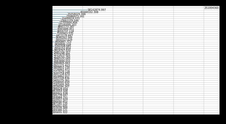
特征重要性画图
1 lgb.plot_importance(
2     gbm,
3     max_num_features=50,
4     importance_type=‘gain‘,
5     figsize=(12,8));
用训练好的模型,再预测test数据,得到submission的csv。
1. 难点
1)特征挖掘,发现隐藏的数据特征,例如城市、商品类别、月份等进行拆分组合。
2)特征融合,不同特征之间的融合,创造新的特征,例如城市、商品的售量平均的过往1-3个月分别作为新特征。
3)时序特征,要瞬移n个月前的数据到当前月。
4)数据的自己补充,item_id与shop_id的全组合才构建出完整的表。要想到只有卖出的才有记录这个点。
5)模型的选择,感觉一般回归的问题,更偏向选择传统机器学习模型吧。像这种很多类别,又是回归的问题,首先想到的就是树模型了。XGboost,lightgbm。感觉效果差不太多吧。因为之前做过一个洛杉矶房价的项目用的就是xgboost,所以这次就想选lightgbm试试。
2. 过程
1)查看数据 --> 2)挖掘数据,发掘更多有用特征 --> 3)融合数据 --> 4)融合特征并制作lag feature --> 5)训练模型,根据预测结果的提升或下降,再调整数据特征。
3. 我的尝试过程
1). 表一开始没补全,loss 20多。太可怕了比sample submission多这么多。。补全后降到了1.多,排名大概top 60%
2). 剪掉item_cnt_month> 2 的,loss降到了0.94,大概top40%
3). 从lag 6个月变成lag 3个月,树模型中feature_name_indexes从放全部类别特征到只放部分类别特征。loss降到了0.93,进步感觉不大,没提交。
4). 加更多特征,例如item_city_month,并且在item_category、shop_name中合并了几个相似的,loss降到了0.90955,No. 1717,大概20%。
5)加更多更多特征,包括一些价格趋势的特征。loss降到了0.894左右。排名大概8%,终于进10%了。(●‘?‘●)
对训练验证数据集还进行过一些尝试,但没啥用的总结:
1)训练全部数据包括第33个月的数据,然后val还是第33个月的数据。
因为觉得第33个月的数据没用上很浪费,所以想试下。而且潜意识也希望模型能更专注更接近第34个月的第33个月的一些数据特征。但很显然这样做会导致过拟合第33个月的数据特征。所以虽然训练时的loss和val loss都下降,但提交后还是0.91左右的loss
2)训练全部数据,val前一年11月的。
因为想着11月可能都会有某些特性,但是因为去年和今年的商品售价等都会有不少的变化,而且也会过拟合去年11月的数据。
那么我如何反映去年11月和我要预测的第34个月,是同一个月呢?于是就想到了加上month这个特征。
4. 总结
1)特征还是更重要。
也许还可以提升的一些思路:
1) 由特征图可以看到,后面一半特征看起来都没啥用,可以尝试去掉后再训练过一次,看是否会有提升。
2)对shop_item的组合加一个 是否出售过该商品的特征。
3)用在train和test中同时出现过的item_id来训练模型,但是这样会不会损失掉一些通用特征呢?需要测试一下。
4)看了一些博主的思路:
4.1 最后提交的结果时,将近12个月没有销量的商品直接置为0.
4.2 将结果中,在train中从未出现过的item的销量直接置为0. (感觉有点粗暴)
4.3 对于新商店,如shop_id=36,直接用第33个月预测第34个月。
4.4 对已关闭的商店,如0,1,8,11,...直接在训练集里去掉这些数据。
4.5 加一些节日的特征,如圣诞节0或1。(但是我感觉月份里面已经反映了这个信息了)
*** 最近太忙了,上面这些还未来得及尝试。等有时间,再试一下,看评分是否会提升。
原文:https://www.cnblogs.com/YeZzz/p/13574801.html
