1.t-SNE

知乎

• t-分布领域嵌入算法
• 虽然主打非线性高维数据降维，但是很少用，因为
• 比较适合应用于可视化，测试模型的效果
• 保证在低维上数据的分布与原始特征空间分布的相似性高

因此用来查看分类器的效果更加

1.1 复现demo

# Import TSNE
from sklearn.manifold import TSNE 

# Create a TSNE instance: model
model = TSNE(learning_rate=200)

# Apply fit_transform to samples: tsne_features
tsne_features = model.fit_transform(samples)

# Select the 0th feature: xs
xs = tsne_features[:,0]

# Select the 1st feature: ys
ys = tsne_features[:,1]

# Scatter plot, coloring by variety_numbers
plt.scatter(xs,ys,c=variety_numbers)
plt.show()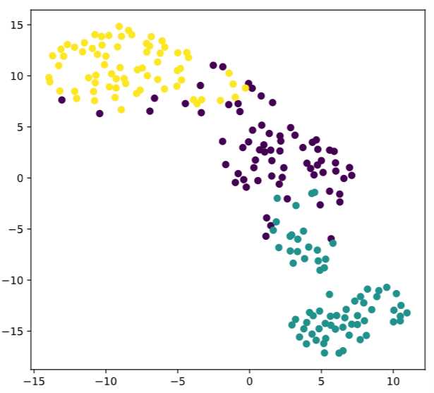

2.PCA

• 当特征变量很多的时候，变量之间往往存在多重共线性。
• 主成分分析,用于高维数据降维，提取数据的主要特征分量
• PCA能“一箭双雕”的地方在于
  • 既可以选择具有代表性的特征，
  • 每个特征之间线性无关
  • 总结一下就是原始特征空间的最佳线性组合
    有一个非常易懂的栗子知乎

2.1 数学推理

可以参考【机器学习】降维——PCA（非常详细）
Making sense of principal component analysis, eigenvectors & eigenvalues

2.2复现

# Perform the necessary imports
import matplotlib.pyplot as plt
from scipy.stats import pearsonr

# Assign the 0th column of grains: width
width = grains[:,0]

# Assign the 1st column of grains: length
length = grains[:,1]

# Scatter plot width vs length
plt.scatter(width, length)
plt.axis('equal')
plt.show()

# Calculate the Pearson correlation
correlation, pvalue = pearsonr(width, length)

# Display the correlation
print(correlation)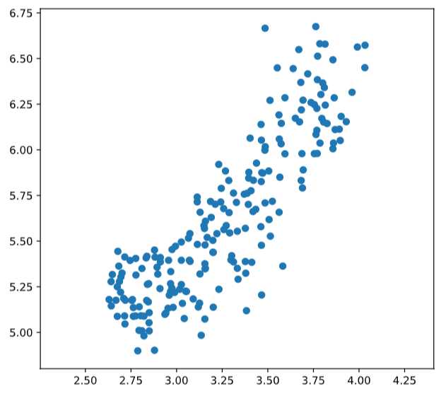

# Import PCA
from sklearn.decomposition import PCA

# Create PCA instance: model
model = PCA()

# Apply the fit_transform method of model to grains: pca_features
pca_features = model.fit_transform(grains)

# Assign 0th column of pca_features: xs
xs = pca_features[:,0]

# Assign 1st column of pca_features: ys
ys = pca_features[:,1]

# Scatter plot xs vs ys
plt.scatter(xs, ys)
plt.axis('equal')
plt.show()

# Calculate the Pearson correlation of xs and ys
correlation, pvalue = pearsonr(xs, ys)

# Display the correlation
print(correlation)

<script.py> output:
    2.5478751053409354e-17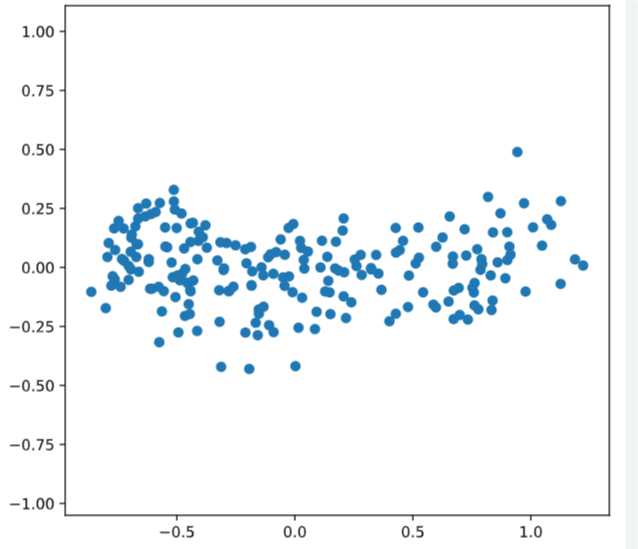

t-SNE and PCA

原文：https://www.cnblogs.com/gaowenxingxing/p/12313864.html