上一节中,我们使用autograd的包来定义模型并求导。本节中,我们将使用torch.nn包来构建神经网络。
一个nn.Module包含各个层和一个forward(input)方法,该方法返回output.
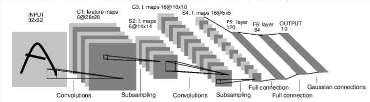
上图是一个简单的前馈神经网络。它接受一个输入。然后一层接着一层地传递。最后输出计算的结果。
神经网络的典型训练过程如下:
# 导入库
import torch
import torch.nn as nn
import torch.nn.functional as F
import torch.optim as optim

# 1 准备数据
# 此处应该替换为数据训练集!!!
input = torch.randn(1, 1, 32, 32)

# 2 创建模型
class Net(nn.Module):  # 定义了一个类,名字叫Net
    注意: 在模型中必须要定义 `forward` 函数,`backward` 函数(用来计算梯度)会被`autograd`自动创建。 可以在 `forward` 函数中使用任何针对 `Tensor` 的操作。

    def __init__(self):  # 每个类都必须有的构造函数,用来初始化该类
        super(Net, self).__init__() # 先调用父类的构造函数
        # 1 input image channel, 6 output channels, 5x5 square convolution
        # kernel
        # 本函数配置了卷积层和全连接层的维度
        self.conv1 = nn.Conv2d(1, 6, 5) # 卷积层1: 二维卷积层, 1个输入通道,6个输出通道, 卷积核大小为5x5
        self.conv2 = nn.Conv2d(6, 16, 5) # 卷积层2: 二维卷积层, 6个输入通道,16个输出通道, 卷积核大小为5x5
        # an affine(仿射) operation: y = Wx + b # 全连接层1: 线性层, 输入维度16*5*5,输出维度120
        self.fc1 = nn.Linear(16 * 5 * 5, 120)
        self.fc2 = nn.Linear(120, 84) # 全连接层2: 线性层, 输入维度120,输出维度84
        self.fc3 = nn.Linear(84, 10) # 全连接层3: 线性层, 输入维度84,输出维度10

    def forward(self, x): #定义了forward函数
        # Max pooling over a (2, 2) window
        x = F.max_pool2d(F.relu(self.conv1(x)), (2, 2)) # 先卷积,再池化
        # If the size is a square you can only specify a single number
        x = F.max_pool2d(F.relu(self.conv2(x)), 2)  # 再卷积,再池化
        x = x.view(-1, self.num_flat_features(x)) # 将x展开成一维(扁平化)
        x = F.relu(self.fc1(x)) # 全连接1
        x = F.relu(self.fc2(x)) # 全连接2
        x = self.fc3(x) # 全连接3
        return x

    def num_flat_features(self, x):
        size = x.size()[1:]  # all dimensions except the batch dimension
        num_features = 1
        for s in size:
            num_features *= s
        return num_features
net = Net()
print(net)

# 3 定义损失函数
criterion = nn.MSELoss()

# 4 初始化:清缓存,求梯度,设置优化器
net.zero_grad()     # zeroes the gradient buffers of all parameters
print('conv1.bias.grad before backward')
print(net.conv1.bias.grad)
loss.backward()
print('conv1.bias.grad after backward')
print(net.conv1.bias.grad)

# create your optimizer
optimizer = optim.SGD(net.parameters(), lr=0.01)  #list(net.parameters())会给出一个参数列表,记录了所有训练参数(W和b)的数据

# 5 训练:
global_step = 10000
for step in range(global_step):
    optimizer.zero_grad()   # zero the gradient buffers
    output = net(input) # 将自动调用Net类里的forward函数,对input设计矩阵进行计算,把返回的Tensor赋给output
    # target = torch.randn(10)  # a dummy target, for example
    target = # 数据集的标签
    target = target.view(1, -1)  # make it the same shape as output
    loss = criterion(output, target)
    params = list(net.parameters())    # net.parameters()返回可被学习的参数(权重)列表和值:
    # print("step:",step,"Weight1",params[0])
    print("step",step,"loss",loss)
    loss.backward()
    optimizer.step()    # Does the update

# 6 打印准确率
# 参考tensorflow部分
除了上面代码段中的实现,你可能还需要了解以下知识:
一个损失函数需要一对输入:模型输出和目标,然后计算一个值来评估输出距离目标有多远。
根据之前学习的理论,一般是计算y和y‘的交叉熵.
例如,对于线性拟合案例,损失函数就是均方误差,即MSE.
output = net(input)
target = torch.randn(10)  # a dummy target, for example
target = target.view(1, -1)  # make it the same shape as output
criterion = nn.MSELoss()

loss = criterion(output, target)
print(loss)
将输出:
tensor(1.3389, grad_fn=<MseLossBackward>)现在,如果你跟随损失到反向传播路径,可以使用它的 .grad_fn 属性,你将会看到一个这样的计算图:
input -> conv2d -> relu -> maxpool2d -> conv2d -> relu -> maxpool2d
      -> view -> linear -> relu -> linear -> relu -> linear
      -> MSELoss
      -> loss
所以,当我们调用 loss.backward(),整个图都会微分,而且所有的在图中的requires_grad=True 的张量将会让他们的 grad 张量累计梯度。
为了演示,我们将跟随以下步骤来跟踪反向传播。
print(loss.grad_fn)  # MSELoss
print(loss.grad_fn.next_functions[0][0])  # Linear
print(loss.grad_fn.next_functions[0][0].next_functions[0][0])  # ReLU
输出:
<MseLossBackward object at 0x7fab77615278>
<AddmmBackward object at 0x7fab77615940>
<AccumulateGrad object at 0x7fab77615940>
为了实现反向传播损失,我们所有需要做的事情仅仅是使用 loss.backward()。你需要清空现存的梯度,要不梯度将会和现存的梯度累计到一起。
现在我们调用 loss.backward() ,然后看一下 con1 的偏置项在反向传播之前和之后的变化。
net.zero_grad()     # zeroes the gradient buffers of all parameters,清空现存的梯度
print('conv1.bias.grad before backward')
print(net.conv1.bias.grad)
loss.backward()
print('conv1.bias.grad after backward')
print(net.conv1.bias.grad)
输出:
conv1.bias.grad before backward
tensor([0., 0., 0., 0., 0., 0.])
conv1.bias.grad after backward
tensor([-0.0054, 0.0011, 0.0012, 0.0148, -0.0186, 0.0087])上面介绍了如何使用损失函数。
最简单的更新规则就是随机梯度下降:weight = weight - learning_rate * gradient。
learning_rate = 0.01
for f in net.parameters():
    f.data.sub_(f.grad.data * learning_rate)
复杂的神经网络参数可这样使用:
import torch.optim as optim

# create your optimizer
optimizer = optim.SGD(net.parameters(), lr=0.01)

# in your training loop:
optimizer.zero_grad()   # zero the gradient buffers
output = net(input)
loss = criterion(output, target)
loss.backward()
optimizer.step() # Does the update原文:https://www.cnblogs.com/charleechan/p/12259781.html