Tushare test

查看版本

import tushare

print(tushare.__version__)

1.2.12

初步的调用方法为：

import tushare as ts
ts.get_hist_data(‘600848‘)  #一次性获取全部日k线数据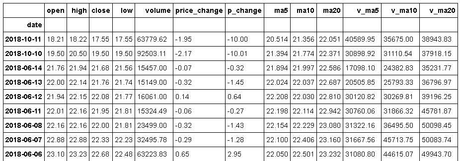

• 第一列是日期，后边的是各类价格，包括开盘价、最高价、收盘价等等，具体在Tushare里边都有详细介绍

调用Tushare抓取上证指数并作可视化

import tushare as ts 
import pandas as pd 
import numpy as np 
import matplotlib.pyplot as plt 

df = ts.get_hist_data(‘000001‘,start=‘2017-01-01‘,end=‘2018-10-10‘) 
df.head(10)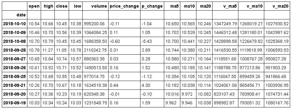

• 可以看到转去了上证指数的各类价格数据以及最后turnover的换手率。但是有一个问题就是数据的date的降序的，即日起从2018年3月往2017年1月排列的，需要排序。

sz=df.sort_index(axis=0, ascending=True) #对index进行升序排列 
sz_return=sz[[‘p_change‘]] #选取涨跌幅数据 
train=sz_return[0:255] #划分训练集 
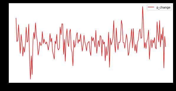
test=sz_return[255:] #测试集 
#对训练集与测试集分别做趋势图 
plt.figure(figsize=(10,5)) 
train[‘p_change‘].plot() 
plt.legend(loc=‘best‘) 
plt.show() 
plt.figure(figsize=(10,5)) 
test[‘p_change‘].plot(c=‘r‘) 
plt.legend(loc=‘best‘) 
plt.show()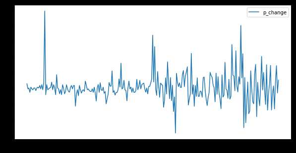

• 蓝色为训练集序列波动图，红色为测试集序列波动图。

直接用训练集平均值作为测试集的预测值

#Simple Average 
from math import sqrt
from sklearn.metrics import mean_squared_error

y_hat_avg = test.copy() #copy test列表 
y_hat_avg[‘avg_forecast‘] = train[‘p_change‘].mean() #求平均值 
plt.figure(figsize=(12,8)) 
plt.plot(train[‘p_change‘], label=‘Train‘) 
plt.plot(test[‘p_change‘], label=‘Test‘) 
plt.plot(y_hat_avg[‘avg_forecast‘], label=‘Average Forecast‘) 
plt.legend(loc=‘best‘) 
plt.show() 
rms = sqrt(mean_squared_error(test.p_change, y_hat_avg.avg_forecast)) 
print(rms)

2.1722839490457657

直接用移动平均法最后一个值作为测试集的预测值

#Moving Average 
from math import sqrt
from sklearn.metrics import mean_squared_error

y_hat_avg = test.copy() 
y_hat_avg[‘moving_avg_forecast‘] = train[‘p_change‘].rolling(30).mean().iloc[-1] 
#30期的移动平均，最后一个数作为test的预测值 
plt.figure(figsize=(12,8)) 
plt.plot(train[‘p_change‘], label=‘Train‘) 
plt.plot(test[‘p_change‘], label=‘Test‘) 
plt.plot(y_hat_avg[‘moving_avg_forecast‘], label=‘Moving Average Forecast‘) 
plt.legend(loc=‘best‘) 
plt.show() 
rms = sqrt(mean_squared_error(test.p_change, y_hat_avg.moving_avg_forecast)) 
print(rms)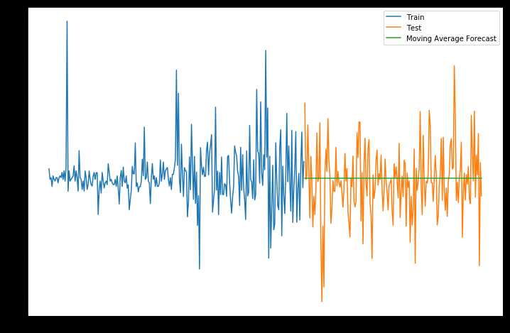

2.1545970719308243

• 得到RMSE为2.1545970719308243

可以看到，最后移动平均法的均方误差最低，预测效果最好。

Tushare test

原文：https://www.cnblogs.com/hankleo/p/9939725.html