本编博客继续分享简单的机器学习的R语言实现。
今天是关于简单的线性回归方程问题的优化问题
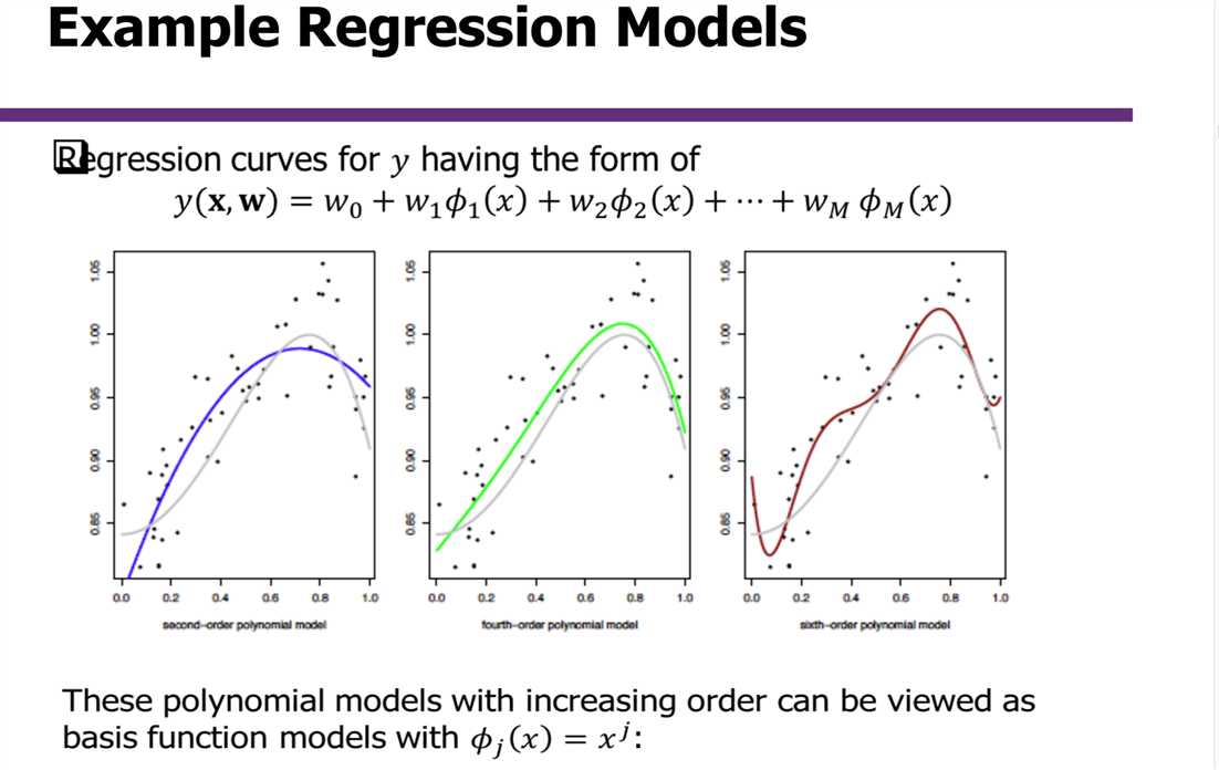
常用方法,我们会考虑随机梯度递降,好处是,我们不需要遍历数据集中的所有元素,这样可以大幅度的减少运算量。
具体的算法参考下面:
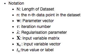
首先我们先定义我们需要的参数的Notation
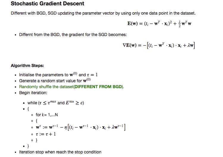
上述算法中,为了避免过拟合,我们采用了L2的正则化,在更新步骤中,我们会发现,这个正则项目,对参数更新的影响
下面是代码部分:
## Load Library
library(ggplot2)
library(reshape2)
library(mvtnorm)

## Function for reading the data
read_data <- function(fname, sc) {
   data <- read.csv(file=fname,head=TRUE,sep=",")
   nr = dim(data)[1]
   nc = dim(data)[2]
   x = data[1:nr,1:(nc-1)]
   y = data[1:nr,nc]
   if (isTRUE(sc)) {
      x = scale(x)  ## Scale x
      y = scale(y)  ## Scale y
   }
   return (list("x" = x, "y" = y))
}
我们定义了一个读取数据的方程,这里,我们会把数据集给scale一下,可以保证进一步提高运算速度
## Matrix Product Function
predict_func <- function(Phi, w){
    return(Phi%*%w)
}

## Function to compute the cost function
train_obj_func <- function (Phi, w, label, lambda){
    # Cost funtion including the L2 norm regulaztion
    return(.5 * mean((predict_func(Phi, w) - label)^2) + .5 * lambda * t(w) %*% w)
}

## Return the errors for each iteration
get_errors <- function(data, label, W) {
    n_weights = dim(W)[1]
    Phi <- cbind(‘X0‘ = 1, data)
    errors = matrix(,nrow=n_weights, ncol=2)
    for (tau in 1:n_weights) {
       errors[tau,1] = tau
       errors[tau,2] = train_obj_func(Phi, W[tau,],label, 0) ## Get the errors, set the lambda to 0
    }
   return(errors)
}
同时,我们定义了计算矩阵乘法,计算目标函数以及求误差的方程。
sgd_train <- function(train_x, train_y, lambda, eta, epsilon, max_epoch) {

    ## Prepare the traindata
    ## Attach the 1 for X0
    Phi <- as.matrix(cbind(‘X0‘=1, train.data))

    ## Calculate the max iteration time for the SGD
    train_len = dim(train_x)[1]
    tau_max = max_epoch * train_len

    W <- matrix(,nrow=tau_max, ncol=ncol(Phi))
    set.seed(1234)
    ## Random Generate the start parameter
    W[1,] <- runif(ncol(Phi))

    tau = 1 # counter
    ## Create a dateframe to store the value of cost function for each iteration
    obj_func_val <-matrix(,nrow=tau_max, ncol=1)
    obj_func_val[tau,1] = train_obj_func(Phi, W[tau,],train_y, lambda)

    while (tau <= tau_max){

        # check termination criteria
        if (obj_func_val[tau,1]<=epsilon) {break}

        # shuffle data:
        train_index <- sample(1:train_len, train_len, replace = FALSE)

        # loop over each datapoint
        for (i in train_index) {
            # increment the counter
            tau <- tau + 1
            if (tau > tau_max) {break}

            # make the weight update
            y_pred <- predict_func(Phi[i,], W[tau-1,])
            W[tau,] <- sgd_update_weight(W[tau-1,], Phi[i,], train_y[i], y_pred, lambda, eta)

            # keep track of the objective funtion
            obj_func_val[tau,1] = train_obj_func(Phi, W[tau,],train_y, lambda)
        }
    }
   # resulting values for the training objective function as well as the weights
    return(list(‘vals‘=obj_func_val,‘W‘=W))
}

# updating the weight vector
sgd_update_weight <- function(W_prev, x, y_true, y_pred, lambda, eta) {
   ## Computer the Gradient
   grad = - (y_true-y_pred) * x
   ## Here I just combine the regularisation term with prev w
   return(W_prev*(1-eta * lambda) - eta * grad)
}
根据上述我们写的计算更新目标函数和参数的方法,讲算法用R实现
下面是实验部分
## Load the train data and train label
train.data <- read_data(‘assignment1_datasets/Task1C_train.csv‘,TRUE)$x
train.label <- read_data(‘assignment1_datasets/Task1C_train.csv‘,TRUE)$y
## Load the testdata and test label
test.data <- read_data(‘assignment1_datasets/Task1C_test.csv‘,TRUE)$x
test.label <- read_data(‘assignment1_datasets/Task1C_test.csv‘,TRUE)$y

# Set MAX EPOCH

max_epoch = 18

## Implement SGD with Ridge regression
options(warn=-1)

## Initilize
## Set the related parameters
epsilon = .001 ## Terimation threshold
eta = .01 ## Learning Rate
lambda= 0.5 ## Regularisation parmater


## Run SGD
## Cost function values
train_res2 = sgd_train(train.data, train.label, lambda, eta, epsilon, max_epoch)
## Calulate the errors
## To be mentioned here, we will only visulisation for the train error to check the converge result
errors2 = get_errors(train.data, train.label, train_res2$W)
接着,我们把SGD的error plot给绘制出来
## Visulastion for SGD
plot(train_res2$val, main="SGD", type="l", col="blue",
     xlab="iteration", ylab="training objective function")

这里我们的方程比较简单,可以看到,目标函数很快就收敛了。
原文:https://www.cnblogs.com/chenyusheng0803/p/9657049.html